[데이콘] 타이타닉 생존자 예측 (캐글 Titanic Machine Learning) (① EDA, 시각화)
[데이터]
PassengerId : 탑승객 고유ID
Survived : 생존유무(0 사망, 1생존)
Pclass : 등실의 등급
Name
Sex
Age
SibSp : 함께 탑승한 형제자매, 아내, 남편의 수
Parch : 함께 탑승한 부모, 자식의 수
Ticket : 티켓번호
Fare : 티켓요금
Cabin : 객실번호
Embarked : 배에 탑승한 위치(Cherbourg, Queenstown, Southampton)
[목표]
탑승객의 데이터를 이용해 생존여부 예측하기
[평가지표]
AUC (area under curve)
본 포스팅에서는
시각화를 익힐 겸 데이터를 천천히 뜯어보기로 하자!
우선 데이터 불러오기
import warnings
warnings.filterwarnings('ignore')

import matplotlib as mpl
import matplotlib.pyplot as plt
%matplotlib inline
plt.rcParams['font.family'] = 'Malgun Gothic'
mpl.rcParams['axes.unicode_minus'] = False

import seaborn as sns
import pandas as pd
train = pd.read_csv(r"./data/train.csv", encoding='utf-8')
test = pd.read_csv(r"./data/test.csv", encoding='utf-8')
submission = pd.read_csv(r"./data/submission.csv", encoding='utf-8')print(train.shape)
print(test.shape)
print(submission.shape)
(891, 12)
(418, 11)
(418, 2)
> 탑승객은 총 418명이구나
train.isna().sum()PassengerId 0
Survived 0
Pclass 0
Name 0
Sex 0
Age 177
SibSp 0
Parch 0
Ticket 0
Fare 0
Cabin 687
Embarked 2
> 결측치 확인. Cabin 데이터는 못쓸 것 같아...☆
1. Survived : 생존유무(0 사망, 1생존)
train['Survived'].value_counts()0 549
1 342
fig, ax = plt.subplots(1,2, figsize=(7,4)) #도화지
labels = ['사망','생존']

train['Survived'].value_counts().plot.bar(ax=ax[0], color='g', rot=0)
ax[0].set(xlabel='Survived', xticklabels=labels, ylabel = 'Count', title = '탑승객 중 사망/생존자 수')

train['Survived'].value_counts().plot.pie(ax=ax[1], startangle=90,
                                          autopct='%.1f%%', fontsize=13, labels=labels)
ax[1].set(title = '탑승객 사망/생존 비율', ylabel = '')
2. Pclass : 등실의 등급
train.groupby('Pclass').mean()['Survived']1 0.629630
2 0.472826
3 0.242363
> 객석 등급별로 생존율에 차이가 있네
fig, ax = plt.subplots(1,3, figsize=(10,4)) #도화지

train['Pclass'].value_counts().sort_index().plot.bar(ax=ax[0], color='g', rot=0)
ax[0].set(title = 'Pclass별 탑승객 수', xlabel='Pclass')

train[['Pclass', 'Survived']].groupby(['Pclass']).mean().plot.bar(ax=ax[1], color='g', rot=0)
ax[1].set(title = 'Pclass별 생존률')

sns.countplot(hue='Survived', x='Pclass', ax=ax[2], data=train)
ax[2].set(title = 'Pclass별 생존/사망자 수')
ax[2].legend(labels=['사망','생존'])
> 3클래스를 이용한 탑승객이 가장 많고, 생존률은 1클래스가 가장 높다.
3. Sex : 탑승객 성별
fig, ax = plt.subplots(2,2, figsize=(8,8))

train['Sex'].value_counts().plot.bar(ax=ax[0,0], rot=0)
ax[0,0].set(xlabel='', title='탑승객 수')

train['Sex'].value_counts().plot.pie(ax=ax[0,1], autopct='%1.1f%%',fontsize=15, startangle=90)
ax[0,1].set(ylabel='', title='탑승객 성비')

sns.countplot(hue='Survived', x='Sex', ax=ax[1,0], data=train)
ax[1,0].set(xlabel='', ylabel='', title = '성별 생존/사망자 수')
ax[1,0].legend(labels = ['사망','생존'])

train[['Sex','Survived']].groupby('Sex').mean().sort_index(ascending=False).plot.bar(ax=ax[1,1], rot=0)
ax[1,1].set(xlabel='', title = '생존률')

> 탑승객 수는 남자가 많았으며, 생존률은 여성이 더 높다.
value_counts() 결과를 컬럼 순서대로 정렬하기 https://hjryu09.tistory.com/51
4. Age : 탑승객 나이
ax = train['Age'].plot.hist(bins=20, rwidth=0.8, title='탑승객의 연령분포')
ax.set(xlabel='age', ylabel='')
# bins 범주 개수
# 또는 seaborn
ax = sns.distplot(train['Age'], bins=20)
ax.set(title='탑승객의 연령분포')
> 20~30대의 탑승객이 많다
5. SibSp : 함께 탑승한 형제자매/아내/남편의 수
Parch : 함께 탑승한 부모/자식의 수
fig, ax = plt.subplots()
ax = train['SibSp'].value_counts().sort_index().plot.bar(rot=0)
ax.set(xlabel='함께 탑승한 형제자매/아내/남편의 수')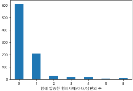
fig, ax = plt.subplots()
ax = train['Parch'].value_counts().sort_index().plot.bar(rot=0)
ax.set(xlabel='함께 탑승한 부모/자식의 수')
> 혼자 탑승한 사람이 많다
# 형제자매, 아내, 남편, 부모, 자식 합산
train['F'] = train['SibSp'] + train['Parch']
train[['F','Survived']].groupby(['F']).mean().plot.bar(rot=0, xlabel='동행한 가족 수', ylabel='생존률')
6. Fare : 티켓요금
train.plot.scatter(x='Pclass', y='Fare', s=5)
> 1클래스가 상대적으로 비싼 티켓이구나
train[['Fare','Pclass']].groupby('Pclass').mean()

> 티켓요금 평균을 비교하면 1클래스 > 2클래스 > 3클래스
7. Embarked : 배에 탑승한 위치
train['Embarked'].unique()['S', 'C', 'Q', nan]
train['Embarked'].value_counts()S 644
C 168
Q 77
fig, ax = plt.subplots(facecolor='white')
train['Embarked'].value_counts().plot.pie(ax=ax, startangle=90, autopct='%.1f%%',
                                          fontsize=15, labels=['S','C','Q'])
ax.set(title='탑승 위치', ylabel='')
티켓번호, 객실번호 등은 .unique() 으로 살펴보고 인사이트를 얻지 못함.